Abstract. The dominating sensor systems for outdoor localization are GNSS (Global Navigation Satellite System) receivers. Due to limited power consumption, small construction size, and low costs GNSS devices are embedded in most of non-autonomous vehicles (airplanes, cars, boats), autonomous systems (robots, drones, etc.) and mobile devices (smart phones, tablets). A single GNSS device provides a localization precision from 1 to 300 m, depending on the number of satellites, their geometrical configuration, and the current disturbance level. Unfortunately this kind of localization is most error prone in urban environments, because shading effects caused by buildings negatively influence localization accuracy.

This is especially problematic when one considers that many future applications based on UAVs (Unmanned Aerial Vehicles) are intended to operate in complex 3D environments, where precise and accurate position estimation is a prerequisite. In order to cope with vague and varying GNSS localization qualities, we have developed a system that can predict the localization uncertainty for a requested space, time, and resolution with different quality metrics.

Authors: André Dietrich & Sebastian Zug

0. Demo

1. Introduction

Most present day localization tasks for manned or unmanned intelligent vehicles are equipped with receivers for at least one Global Navigation Satellite Systems (GNSS). The ubiquity is reasonable, due to the fact that modern GNSS devices are cheap, small in size, have a low-energy consumption, and provide position information with a maximum uncertainty of 300 m for each position on or near earth. The continuous modernization of the U.S. Global Positioning System (GPS), the new European Galileo satellite system, Russian GLONASS, Chinese BeiDou, and the launch of quasi-zenith satellites by Japan illustrate the increased importance of an omnipresent position information.

Because of the previously mentioned maximum uncertainty level, most of today’s GNSS receivers are embedded in a multi-modal sensor system for (semi-)autonomous, automotive scenarios. GNSS measurements and inertial measurements are fused with camera and odometry data in order to provide more precise localization and speed information. In Section 2 we give a comprehensive overview of commonly applied approaches for improving localization quality based on GNSS measurements. These concepts provide only vague or not applicable improvements for near future scenarios in urban environments, such as delivery services based on Unmanned Aerial Vehicles (UAVs), as intended by Amazon PrimeAir [1], Google Wing [2], DHL Parcelcopter [3], the DomiCopter [4] and TacoCopter [5] projects (for fast food delivery), even first aid drones [6], or autonomous systems for law enforcement, surveillance, traffic monitoring, evaluation of accident scenes [7], etc. Here we have to guarantee a certain localization accuracy for all points of a 3D-trajectory too. UAVs operating in urban environments have to fulfill higher safety requirements, while state of the art mechanisms can only be applied partly or not at all. The power consumption and construction space are the limiting factors for additional sensors, whereby external disturbances (e. g., wind, rain, dust) and the number of degrees of freedom (depending on the UAV type) make the localization much more difficult. For this purpose we present a new kind of GNSS forecasting service for urban scenarios, which is currently implemented for GPS only. It can be used for localization oriented path planning, GNSS signal selection and filtering, and thus for minimizing localization uncertainties.

3.1 Our Approach

gments 3D geometrical representations of the environment with predicted GNSS information for a certain time or period of time. This new abstraction can be used to answer questions according to reliable localization quality, based on GNSS measurements, like:

• “What is the best time to perform a flight on a certain trajectory?”

• “At which height level does a UAV have to operate corresponding to a certain point in time and space?”

• “What is the optimal combination of satellite signals for a position estimation for a certain area and time?”

• “What is the average/minimal/deviation of/... localization quality in that region?”

For this purpose, we gather landscape and building geometries as well as status information about satellites from different web sources to predict the shading effects caused by the environment on GNSS measurements for a certain point in time and space, determine satellite visibility and calculate the corresponding localization quality.

The picture above shows an aerial view of Manhattan representing the GPS dilution of precision (DOP). This quality metric (which will be discussed in detail in Section 3.3) forms canyons and valleys between buildings with varying localization precisions. New kinds of 4D path planning algorithms can be applied on these representations to optimize flight trajectories, heights, energy consumptions, etc.

1.2 Overview

In the next section we discuss concepts for improving the quality of GNSS measurements and discuss the benefits of our approach, based on environmental context information (gained from highly accurate 3D models). In Section 3 we describe our concept in detail and outline each of the challenging tasks to be accomplished. The section contains and discusses furthermore the initial results, which is followed by a conclusion and an outlook for future works.

2. Related Work

Path planning algorithms considering the expected localization quality are already described for different robot domains and sensor systems [8], [9]. The scenarios described are often bound to a certain sensor type and environment. Nevertheless, the basic concept is always the same, beside the existing environment model an additional prediction and representation of the localization uncertainty is needed [10]. A comprehensive overview on trajectory planning methods for such uncertain environments is given by Jun, Chaudhry, and D’Andrea in [11].

Our mapping method includes a quality information for GNSS measurements and depends on appropriate metrics to represent them. Related errors and their sources for GNSS localization are discussed in detail in [12]. The effect on the localization quality is covered by a large number of studies [13], [14], which derive an associated statistical quality assessment. A corresponding probabilistic uncertainty is suitable to express the capabilities of a GNSS receiver in general, but it does not answer the question of the specific localization quality for a certain point.

GNSS receivers fuse individual distance measurements and calculate a position estimation. The effects of the above mentioned errors strongly depend on the geometric configuration of the satellite orbits and is described by the Dilution of Precision (DOP) in [15]. Wang, Groves, and Ziebart evaluated the DOP for small area in London. The authors furthermore revealed that a reliable localization is not possible for a lot of urban positions. The is DOP above a minimum threshold (we explain this issue in detail in Section 3.3.2) for 12 to 22 % of the evaluated positions [16]. Another study, presented in [15], discussed the fluctuation of DOP values over 24 hours and Milbert presented a detailed analysis of DOP and introduced DOP-maps in [17].

Beside the actual configuration of the GNSS, the situational context on Earth affects the quality of position estimations too. For urban scenarios in particular, the uncertainty increases due to the fact that the number of satellites in the line-of-sight is reduced [18]. The corresponding signals do not reach the receiver or get reflected from walls. Many papers address this problem and present different solutions, the most relevant paper [19] in this context was written by Wang, Groves, and Ziebart. The authors had implemented a tool-chain to evaluate the quality of GNSS signals with the help of a 3D city model. It was used to identify satellites in line-of-sight and at the end to improve GNSS predictions. An infrared camera system was applied in [20] to capture the surrounding skyline before calculating a position. The skyline was used to identify invisible satellites, which were excluded from the position calculation. The authors could show a significant improvement of the localization quality (for one specific position). Position estimations for buses were improved in [21] by context information about road map and the typical routes. Based on the assumption that devices are moving on a street, GNSS outputs can be weighted respectively. Other approaches evaluate signal characteristics like the signal strength in [22] or the different polarizations of reflected and direct line-of-sight signals [23].

All of the methods mentioned above are related to GNSS measurements and are focused on an online-improvement of the localization quality. In essence, this goal can be reached only by integrating additional sensors. In order to avoid associated costs and energy consumption we shift the effort to a pre-flight offline planning phase by predicting the GNSS localization accuracy with different quality metrics.

3 GPS Forecasting

3.1 Implementation & Sources

The diagram in Fig. 1 comprises all components of our implementation as well as all tapped data sources. A configuration file contains all necessary parameters, these are the location, time, and resolution of the measurement.

The DataGrabber is applied to gather all required information for a specific region. The main source is the web-api of Open Street Maps (OSM), which allows the possibility of selectively downloading maps in an OSM-XML format. It contains information about buildings, streets, traffic signs, places of interest, etc. In contrast to Google-Earth, OSM is an openly licensed map that is continuously updated by volunteers using local knowledge, GPS tracks, and donated sources. Due to the open data initiative there is a growing number of donations from various land registry offices and governmental institutions, especially in Europe. The high accuracy of OSM is also underpinned by the study in [24], at least for Germany. This data can be combined with SRTM files, which stands for Shuttle Radar Topography Mission and contains topological elevation information, to generate high-resolution 3D models with the help of OSM2World. The Bing web-api is applied to automatically retrieve satellite images, the minimum altitude of the terrain, and the central map coordinates. A continuously updated list of operational satellites (OPS) that describes their current state (position, velocity, inactivity) is retrieved from the Center for Space Standards & Innovation (which operates the satellite tracking web site CelesTrak).

All of this information in conjunction with the generated 3D model is used as input for our Scanner module (see also the screenshot in Fig. 2). It combines our odeViz library with the pyephem. odeViz is used to as a wrapper for ODE (Open Dynamics Engine) simulations and automatically sets up the appropriate visualization with VTK (Visualization Toolkit). pyephem is a package for performing high precision astronomy computations.

3.2 Line-of-Sight Analysis

Related to the physical operating principle, the availability is limited by the need for an unobstructed line-of-sight on at least four GNSS satellites. At least three satellite signals are necessary to solve the equation system related to the requested position (longitude, latitude, and altitude). An additional signal has to be evaluated due to the uncertainty of the receiver clock. For the GPS system each position is theoretically covered by up to twelve satellites simultaneously. The duration of a satellite orbit above an observer’s horizon depends on its position related to the six main orbital planes.

Due to the low transmission power of the GNSS signals a direct line-of-sight between satellite and receiver is necessary. Consequently, the number of actually available satellites is reduced by geographical conditions (mountains, canyons), vegetation or buildings. This analysis happens within the Scanner module (cf. Fig. 2), which is in fact rigid body simulation, and contains the entire 3D city model. pyephem is applied to determine the relative positions of the GPS satellites according to a certain point within the model and according to a certain point in time. By using rays, which start at a local position and extend in the direction of the satellites, it is possible to check whether a satellite is in line-of-sight or not. If there is no collision detected between the model and the ray, then the satellite should be visible from that position, otherwise not.

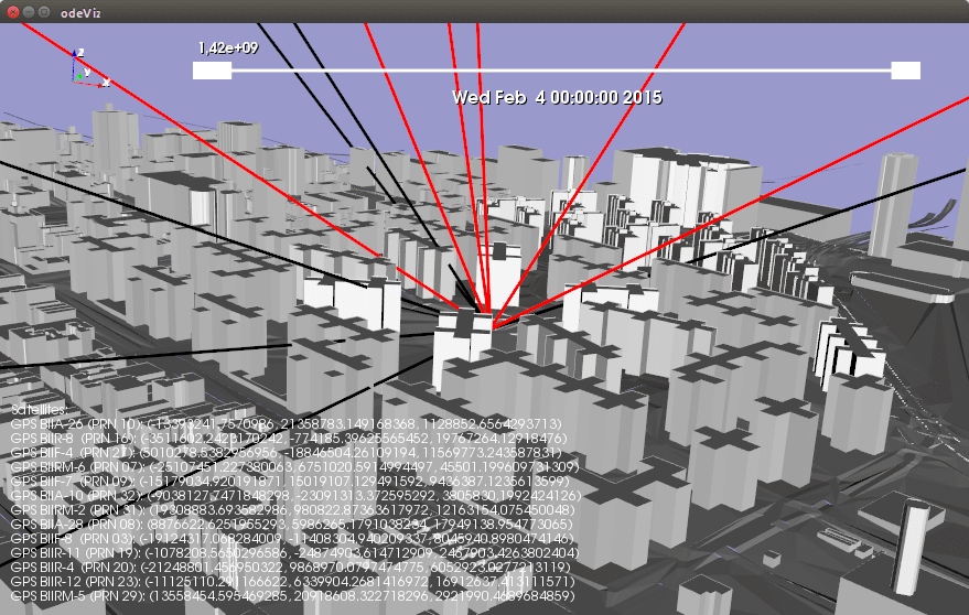
To demonstrate this discrepancy between the number of satellites that should be visible (above horizon) and hidden ones, we chose the the area of Manhattan already depicted in Fig. 2. In contrast to most districts in that region, it contains a free round area, buildings are not posed on a grid like structure, and furthermore the building geometries themselves are more complex than simple cubes. The screenshot in Fig. 3 shows an overlay of our model based-predictions with the results obtained from Trimble (an online GNSS planning tool) for a period of 24 hours. The black stripes indicate that a satellite is above the horizon but not in direct line-of-sight.

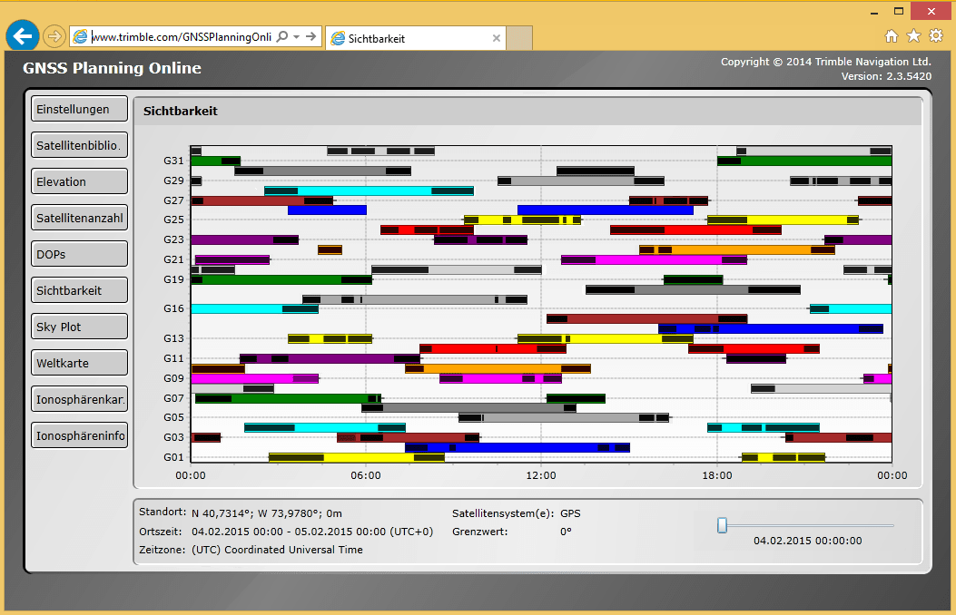
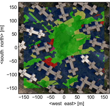
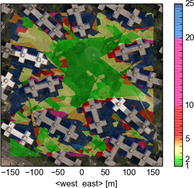
Our predictions matched those of Trimble for the considered GPS location and show that satellites can be out of sight for quite long periods of time, and thus not usable for position estimations, especially during satellite rise and set. Thus, most of the time, the number of visible satellites is much smaller than predicted with common methods. Space is another factor causing fluctuations. Fig. 4 contains two snapshots of a 24-hour analysis (available on our website), which depicts the difference in the number of satellites in line-of-sight in 2D for two different points in time. It is easy to see, that a deviation of one meter can cause a tremendous decrease or increase of available satellite signals.

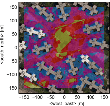
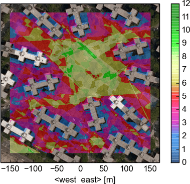
It is primarily the proximity to one of the buildings that causes a reduction of visible satellites, but it has a further consequence (not directly visible in Fig. 4). The geometrical constellation of line-of-sight satellites is poor compared to free space, because satellite signals can only be received from limited angular positions. That causes a decrease in localization quality. Thus, the number of visible satellites cannot be directly applied as a quality metric.

In reality, some of the blocked satellite signals reach the receiver after reflections. The additional transmission length results in so called multi-path-errors and have to be excluded from further processing. Because of the shading effects, some authors have developed multi-GNSS systems that combine the satellites GPS with GLONASS or GALILEO to cope with this problem (cf. [25], [26]). Depending on the position and the level of the horizon, the improvement is significant but can be reached only with additional hardware.

3.3 Quality Metrics

As indicated, the number of visible satellites is a weak quality metric. It does not incorporate the magnitude of localization errors or uncertainty for a certain position, which is caused by a specific satellite constellation.

3.3.1 Distance Errors

For a localization based on a GNSS we evaluate the transient time between satellite and receiver in a first step. Signal propagation is disturbed by atmospheric conditions, satellite ephemeris errors, and clock drifts. The corresponding pseudo-range $\rho_i$ can be calculated by

$$
\rho_i = \rho^T_{i} + c (\delta^s_i - \delta_R) \text{ for } 4 \leq i \leq n
$$

where $\rho^T_{i}$ is the real range from the true position to the $i$th of $n$ satellites [15]. This distance information is overlaid by errors generated by an inaccuracy of the receiver clock ($\delta_R$) and external errors ($\delta_i$) that are related to atmospheric conditions, satellite ephemeris errors, and clock drifts. $c$ stands for the vacuum speed of light. A GNSS receiver has to solve the corresponding equation system to calculate the position $\hat{x}$ with a covariance of $C_{\hat{x}}$ according to

\begin{align}
\label{equ:C}
C_{\hat{x}}=\left(A^T C^{-1}_{\Delta\rho} A\right)^{-1}
\end{align}

$C_{\Delta\rho}$ represents the covariance matrix of the pseudo-range measurements. $A$ is an $n \times 4$ matrix of the partial derivatives of the pseudo-ranges $\rho_i$ with respect to the unknown values for position and time, while $R_{i}$ denotes the euclidean distance between the $i$th satellite and the receiver.

\begin{align}
\label{equ:A}
A =
\begin{pmatrix}
\frac{x_{1}-x}{R_{1}} & \frac{y_{1}-y}{R_{1}} & \frac{z_{1}-z}{R_{1}} & -1 \newline
\vdots & \vdots & \vdots & \vdots \newline
\frac{x_{n}-x}{R_{n}} & \frac{y_{n}-y}{R_{n}} & \frac{z_{n}-z}{R_{n}} & -1
\end{pmatrix}
\end{align}

If we assume a constant error model for all distance measurements with a particular standard deviation $\sigma_{\rho}$, we can define $C_{\hat{x}} = \sigma^2_{\rho}I$, where $I$ represents the identity matrix $n \times n$. Consequently, \eqref{equ:C} can be simplified to

\begin{align}
\label{equ:Csimple}
C_{\hat{x}}=\left(A^T A\right)^{-1} \sigma_{\rho}^2 = D \sigma_{\rho}^2
\end{align}

3.3.2 Dilution of Precision (DOP)

Equation \eqref{equ:C} and \eqref{equ:Csimple} show an important aspect -- the common error level is defined by the distance errors and a gain ($A$) that represents the geometrical relation of the available satellites. If all satellites are adjusted on a straight line in x-direction for instance, the rows of $A$ are linearly dependent due to $y_i, z_i = const.$ Hence, the position uncertainty based on a certain distance error $\sigma_{\rho}$ is much higher than for an orthogonal deployment of the satellites.

This effect is described by the DOP. It represents the gain of the initial distance error and can be calculated by

\begin{align}
DOP = \frac{\Delta \text{Output Location}}{\Delta \text{Measured Data}}
\end{align}

If we follow the idea of a constant non-correlated $\sigma_{\rho}$ for each satellite, the DOP is a suitable abstraction to compare relatively the GNSS localization quality for specific points and times [27]. DOP values can be calculated for different contexts. The horizontal HDOP addresses the effect of the satellite configuration on the latitude and longitude values. The VDOP focuses on the altitude quality, whereas the positional PDOP includes all three localization aspects [15]. The values can be calculated by

\begin{align}
\text{HDOP} &= \frac{\sigma_H}{\sigma_{\rho}} = \sqrt{D_{11} + D_{22}} \nonumber\newline
\text{PDOP} &= \frac{\sigma_P}{\sigma_{\rho}} = \sqrt{D_{11}+D_{22}+D_{33}}
\end{align}

In the case of an optimal satellite constellation the measurement error is notextended and consequently we receive a DOP of $1$. Worst-case scenarios generate much higher values. Tab. 1 summarizes the consequences of DOP values based on the maximum error level for $\sigma_{\rho}$. A DOP value larger than $20$ indicates that the between the GNSS measurement and the true position deviates by more than 300 m.

Tab. 1: DOP-rating for GNSS measurements [17], [27]

DOP	Rating	Description
1	Ideal	The highest possible precision at all times.
1 − 2	Excellent	Positional measurements are considered as accurate enough to meet the most sensitive applications.
2 − 5	Good	Positions fulfill the uncertainty demands of inroute navigation suggestions.
5 − 10	Moderate	Measurements have a limited quality. A more open view of the sky is recommended.
10−20	Fair	Position measurements indicate only a very rough estimate of the location.
> 20	Poor	At this level, the uncertainty reaches a nontolerable level, the measurements should be discarded.

While GNSS receivers provide run-time DOP values for specific locations, we can now pre-calculate the DOPs for a complete area. The corresponding HDOPs for the scenarios depicted in Fig. 5 are visible in the diagrams below. At most positions between the 13-floor buildings the HDOP is high (dark blue, $\text{HDOP} > 20$), a localization based on GPS measurements is thus not possible or reliable there. The situation changes at noon, where the area with a $\text{HDOP}<5$ increases, due to the fact that fewer satellites are hidden behind buildings and that they are in a better geometrical configuration. Consequently, at different points in time we can find passages between the buildings with good localization qualities.

3.3.3 4D-Mapping

The HDOP values in Fig. 5a and 5b were calculated at ground level and passages become visible at different points in time. Now, imagine we would lift up, the number of hidden satellites would automatically decrease, resulting in better DOPs. We can now build 3D maps where good DOPs form canyons between buildings and points with poor localization quality. In contrast to Fig. 5, the image on the first page shows a 3D representation of the PDOP values for Downtown Manhattan (a worst case environment compared to Stuyvesant Town) on 4th of February 2015. The skyline is visible, as is Battery Park in the foreground. The street canyons are overlaid by different layers representing a certain PDOP level.

Based on our GPS weather forecasts, we should be able to determine trajectories within such DOP canyons that guarantee a high localization quality at all positions. Localization information has to be combined with energy consumptions aspects. The ascent and descent to different altitudes consumes energy and extends the trajectory length for a UAV. But in contrast to most common trajectory planning algorithms we also have to deal with time as the 4th dimension. Passages with good DOPs are only open for a certain period of time. The calculated trajectories to a destination point and back can thus be completely different.

4. Conclusion & Outlook

In this paper we defined a new map representation for drones path planning that combines 3D building information with an expected localization quality based on GNSS measurements at each position. We described the sources and the work flow to generate the 3D environment model, the mechanisms to predict the GNSS satellite positions and the calculation of a 3D DOP map. The project achieves this using exclusively open access data and open source software.

With this paper we build the foundation for 4D-DOP based path planning for UAVs. In further steps we want to enhance the project to make it applicable for large-scale scenarios with autonomous robots and UAVs:

• At this point, the uncertainty measure evaluates only the DOP values. They just provide relative comparisons of the localization precision for different positions. We want to implement a more distance oriented error model, which provides an absolute value and considers tropospheric and atmospheric effects.

• OSM-3D includes a large number of plugins and applications for easy access on the available data. The GPS weather forecast should receive the status of an official plugin that provides the predicted uncertainty as a 2D map for driving scenarios. The 3D representation for UAVs will be available in a separate web service.

• As a part of the UAV path planning, we have to derive appropriate cost functions and to select an appropriate 4D algorithm evaluating multiple 3D GNSS maps.

References

[1] G. S. McNeal, “Six Things You Should Know About Amazon’s Drones,” Forbes, Nov. 2014. [Online]. Available: http://www.forbes.com/sites/gregorymcneal/2014/07/11/six-things-you-need-to-know-about-amazons-drones/

[2] BBC News - Techonology, Google tests drone deliveries in Project Wing trials, Online press release, Aug. 2014. [Online]. Available: http://www.bbc.com/news/technology-28964260

[3] DHL International GmbH, DHL parcelcopter launches initial operations for research purposes, Online press release, Sep. 2014. [Online]. Available: http://www.dhl.com/en/press/releases/releases_2014/group/dhl_parcelcopter_launches_initial_operations_for_research_purposes.html

[4] U.S.News, Drones Have a Future in Deliveries, But Not for Domino’s Pizza, Online press release, Jun. 2013. [Online]. Available: http://www.usnews.com/news/articles/2013/06/06/drones-have-a-future-in-deliveries-but-not-for-dominos-pizza

[5] Huffington Post, Flying Robots Deliver Tacos To Your Location, Online press release, Mar. 2013. [Online]. Available: http://www.huffingtonpost.com/2012/03/23/tacocopter-startup-delivers-tacos-by-unmanned-drone-helicopter_n_1375842.html

[6] Techcrunch, This Ambulance Drone Can Fly Into Trouble With First Aid, Online press release, Oct. 2014. [Online]. Available: http://techcrunch.com/2014/10/31/this-ambulance-drone-can-fly-into-trouble-with-first-aid/

[7] U-T Santiago, Tijuana to use drones, Online press release, Dec. 2013. [Online]. Available: http://www.utsandiego.com/news/2013/dec/07/drones-3D-robotics-tijuana-san-diego-mayor/

[8] H. Takeda, C. Facchinetti, and J.-C. Latombe, “Planning the motions of a mobile robot in a sensory uncertainty field,” IEEE Transactions on Pattern Analysis and Machine Intelligence, vol. 16, no. 10, pp. 1002–1017, 1994.

[9] J. Van Den Berg, P. Abbeel, and K. Goldberg, “LQG-MP: Optimized path planning for robots with motion uncertainty and imperfect state information,” The International Journal of Robotics Research, vol. 30, no. 7, pp. 895–913, 2011.

[10] J. Faigl, T. Krajnık, V. Vonásek, and L. Preucil, “Surveillance planning with localization uncertainty for uavs,” in 3rd Israeli Conference on Robotics, 2010.

[11] M. Jun, A. I. Chaudhry, and R. D’Andrea, “The Navigation of Autonomous Vehicles in Uncertain Dynamic Environments: A Case Study (I),” in IEEE Conference on Decision and Control, IEEE; 1998, vol. 4, 2002, pp. 3770–3775.

[12] B. Hofmann-Wellenhof, H. Lichtenegger, and E. Wasle, GNSS – Global Navigation Satellite Systems: GPS, GLONASS, Galileo, and more. Springer, 2007.

[13] M. Matosevic, Z. Salcic, and S. Berber, “A Comparison of Accuracy Using a GPS and a Low-Cost DGPS,” IEEE Transactions on Instrumentation and Measurement, vol. 55, no. 5, pp. 1677–1683, 2006.

[14] L. L. Arnold and P. A. Zandbergen, “Positional accuracy of the wide area augmentation system in consumer-grade GPS units,” Computers & Geo-sciences, vol. 37, no. 7, pp. 883–892, 2011.

[15] R. B. Langley, “Dilution of Precision,” GPS world, vol. 10, no. 5, pp. 52–59, 1999.

[16] L. Wang, P. D. Groves, and M. K. Ziebart, “Multi-constellation GNSS performance evaluation for urban canyons using large virtual reality city models,” Journal of Navigation, vol. 65, no. 03, pp. 459–476, 2012.

[17] D. Milbert, “Dilution of precision revisited,” Navigation, vol. 55, no. 1, pp. 67–81, 2008.

[18] P. D. Groves, Z. Jiang, L. Wang, and M. Ziebart, “Intelligent urban positioning, shadow matching and non-line-of-sight signal detection,” in 6th ESA Workshop on Satellite Navigation Technologies and European Workshop on GNSS Signals and Signal Processing (NAVITEC), 2012, pp. 1–8.

[19] L Wang, P. Groves, and M. Ziebart, “Urban Positioning on a Smartphone: Real-time Shadow Matching Using GNSS and 3D City Models,” Inside GNSS Magazine, vol. 8, no. 6, pp. 44–56, 2013.

[20] J. Meguro, T. Murata, J. Takiguchi, Y. Amano, and T. Hashizume, “GPS accuracy improvement by satellite selection using omnidirectional infrared camera,” in IEEE/RSJ International Conference on Intelligent Robots and Systems (IROS), IEEE, 2008, pp. 1804–1810.

[21] G. Taylor, C. Brunsdon, J. Li, A. Olden, D. Steup, and M. Winter, “GPS accuracy estimation using map matching techniques: Applied to vehicle positioning and odometer calibration,” Computers, environment and urban systems, vol. 30, no. 6, pp. 757–772, 2006.

[22] T. Matsushita, T. Tanaka, and M. Yonekawa, “Method for accuracy improvement of GPS measurement in the city,” in ICCAS-SICE, 2009, pp. 3966–3969.

[23] P. Groves, Z Jiang, B Skelton, P. Cross, L Lau, Y Adane, and I Kale, “Novel Multipath Mitigation Methods using a Dual-Polarization Antenna,” in Proceedings of the 23rd International Technical Meeting of The Satellite Division of the Institute of Navigation (ION GNSS), 2010, pp. 140–151.

[24] M. Goetz and A. Zipf, “OpenStreetMap in 3D–detailed insights on the current situation in Germany,” in Proceedings of 15th AGILE International Conference on Geographic Information Science, Avignon, France, 2012, pp. 24–27.

[25] A. Bochkovskii, N. Mikhailov, and S. Pospelov, “GPS/GLONASS receiver for consumer market,” English, Gyroscopy and Navigation, vol. 3, no. 3, pp. 181–187, 2012.

[26] P. Mattos, “Consumer GPS/GLONASS: Accuracy and Availability Trials of a One-Chip Receiver in Obstructed Environments,” GPS World, vol. 22, no. 12, Dec. 2011.

[27] G. Seeber, Satellite geodesy: foundations, methods, and applications. Walter de Gruyter, 2003.