Simple check of a sample against 80 distributions
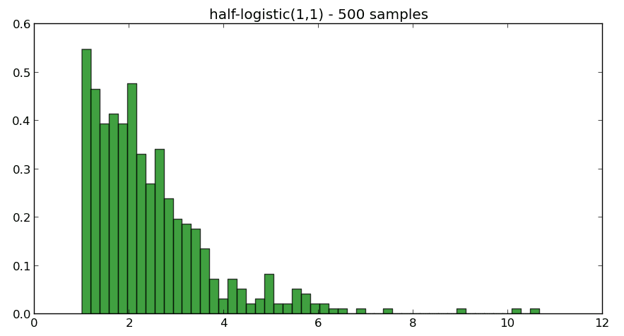
Who ever wanted to check a sample of measurements against different distributions… Here is a quite simple way to do so by using python scipy. We have for example a random sample of 500 values generated with the following command (the complete script can be downloaded at https://github.com/andre-dietrich/distribution-check):
import scipy.stats
sample = scipy.stats.halflogistic(1,1).rvs(500)
The following picture shows a histogram of our sample:
Of course, we know that the distribution is half-logistic, but is it also possible to determine the probability distribution afterwards? Scipy already includes all necessary stuff, firstly here is a list of some available distributions:
cdfs = [
    "norm",            #Normal (Gaussian)
    "alpha",           #Alpha
    "anglit",          #Anglit
    "arcsine",         #Arcsine
    "beta",            #Beta
    "betaprime",       #Beta Prime
    "bradford",        #Bradford
    "burr",            #Burr
    "cauchy",          #Cauchy
    "chi",             #Chi
    "chi2",            #Chi-squared
    "cosine",          #Cosine
    "dgamma",          #Double Gamma
    "dweibull",        #Double Weibull
    "erlang",          #Erlang
    "expon",           #Exponential
    "exponweib",       #Exponentiated Weibull
    "exponpow",        #Exponential Power
    "fatiguelife",     #Fatigue Life (Birnbaum-Sanders)
    "foldcauchy",      #Folded Cauchy
    "f",               #F (Snecdor F)
    "fisk",            #Fisk
    "foldnorm",        #Folded Normal
    "frechet_r",       #Frechet Right Sided, Extreme Value Type II
    "frechet_l",       #Frechet Left Sided, Weibull_max
    "gamma",           #Gamma
    "gausshyper",      #Gauss Hypergeometric
    "genexpon",        #Generalized Exponential
    "genextreme",      #Generalized Extreme Value
    "gengamma",        #Generalized gamma
    "genlogistic",     #Generalized Logistic
    "genpareto",       #Generalized Pareto
    "genhalflogistic", #Generalized Half Logistic
    "gilbrat",         #Gilbrat
    "gompertz",        #Gompertz (Truncated Gumbel)
    "gumbel_l",        #Left Sided Gumbel, etc.
    "gumbel_r",        #Right Sided Gumbel
    "halfcauchy",      #Half Cauchy
    "halflogistic",    #Half Logistic
    "halfnorm",        #Half Normal
    "hypsecant",       #Hyperbolic Secant
    "invgamma",        #Inverse Gamma
    "invnorm",         #Inverse Normal
    "invweibull",      #Inverse Weibull
    "johnsonsb",       #Johnson SB
    "johnsonsu",       #Johnson SU
    "laplace",         #Laplace
    "logistic",        #Logistic
    "loggamma",        #Log-Gamma
    "loglaplace",      #Log-Laplace (Log Double Exponential)
    "lognorm",         #Log-Normal
    "lomax",           #Lomax (Pareto of the second kind)
    "maxwell",         #Maxwell
    "mielke",          #Mielke's Beta-Kappa
    "nakagami",        #Nakagami
    "ncx2",            #Non-central chi-squared
#    "ncf",             #Non-central F
    "nct",             #Non-central Student's T
    "pareto",          #Pareto
    "powerlaw",        #Power-function
    "powerlognorm",    #Power log normal
    "powernorm",       #Power normal
    "rdist",           #R distribution
    "reciprocal",      #Reciprocal
    "rayleigh",        #Rayleigh
    "rice",            #Rice
    "recipinvgauss",   #Reciprocal Inverse Gaussian
    "semicircular",    #Semicircular
    "t",               #Student's T
    "triang",          #Triangular
    "truncexpon",      #Truncated Exponential
    "truncnorm",       #Truncated Normal
    "tukeylambda",     #Tukey-Lambda
    "uniform",         #Uniform
    "vonmises",        #Von-Mises (Circular)
    "wald",            #Wald
    "weibull_min",     #Minimum Weibull (see Frechet)
    "weibull_max",     #Maximum Weibull (see Frechet)
    "wrapcauchy",      #Wrapped Cauchy
    "ksone",           #Kolmogorov-Smirnov one-sided (no stats)
    "kstwobign"]       #Kolmogorov-Smirnov two-sided test for Large N
And finally, there are only two things, which we have to do… fitting our set of sample against every probability distribution and applying the “Kolmogorov-Smirnof one sided test” as follows:
for cdf in cdfs:
    #fit our data set against every probability distribution
    parameters = eval("scipy.stats."+cdf+".fit(sample)");

    #Applying the Kolmogorov-Smirnof one sided test
    D, p = scipy.stats.kstest(sample, cdf, args=parameters);

    #pretty-print the results
    print cdf.ljust(16) + ("p: "+str(p)).ljust(25)+"D: "+str(D);
Running this example, we get the following result:
norm            p: 4.32985784116e-07     D: 0.123361363632
alpha           p: 0.0                   D: nan
anglit          p: 1.57405644075e-09     D: 0.14414705595
arcsine         p: 0.0                   D: 0.194487444742
beta            p: 0.17194522643         D: 0.0492004317884
betaprime       p: 0.0                   D: nan
bradford        p: 2.6871305181e-10      D: 0.150085923622
burr            p: 0.0                   D: nan
cauchy          p: 0.0                   D: nan
chi             p: 0.202823098481        D: 0.0475053082334
chi2            p: 0.0                   D: 0.258
cosine          p: 1.33185751316e-08     D: 0.136622959885
dgamma          p: 1.99526513089e-08     D: 0.135150952901
dweibull        p: 9.10639612606e-08     D: 0.129470516829
erlang          p: 1.55989546051e-05     D: 0.108
expon           p: 1.55989546051e-05     D: 0.108
exponweib       p: 1.55989546051e-05     D: 0.108
exponpow        p: 0.00738341390149      D: 0.0744818772737
fatiguelife     p: 2.64361865732e-10     D: 0.150139654368
foldcauchy      p: 0.0                   D: nan
f               p: 0.0                   D: nan
fisk            p: 0.0                   D: nan
foldnorm        p: 0.0195268210697       D: 0.0676853081311
frechet_r       p: 1.55989546051e-05     D: 0.108
frechet_l       p: 0.0                   D: 0.250852727712
gamma           p: 0.064713393752        D: 0.0582325521395
gausshyper      p: 2.6871305181e-10      D: 0.150085923622
genexpon        p: 0.793140816507        D: 0.0290362909155
genextreme      p: 0.0                   D: 0.250852727712
gengamma        p: 1.55989546051e-05     D: 0.108
genlogistic     p: 0.197774458464        D: 0.0477678936548
genpareto       p: 0.0                   D: nan
genhalflogistic p: 1.11022302463e-15     D: 0.186514196604
gilbrat         p: 0.0                   D: 0.244376114481
gompertz        p: 0.104396819147        D: 0.0540007747394
gumbel_l        p: 0.0                   D: 0.266977935937
gumbel_r        p: 0.191127509048        D: 0.0481217433314
halfcauchy      p: 0.0                   D: nan
halflogistic    p: 0.861779698542        D: 0.0269170250918
halfnorm        p: 0.0196547930831       D: 0.0676373500658
hypsecant       p: 5.24874010255e-07     D: 0.122585921974
invgamma        p: 0.0                   D: nan
invnorm         p: 2.05302441714e-12     D: 0.1653403998
invweibull      p: 0.0                   D: nan
johnsonsb       p: 0.000123301008122     D: 0.0980415299941
johnsonsu       p: 0.187690615262        D: 0.0483085152879
laplace         p: 6.4301079794e-08      D: 0.130794611581
logistic        p: 2.0080315426e-06      D: 0.117035439077
loggamma        p: 2.47024765088e-07     D: 0.125595005169
loglaplace      p: 0.0                   D: nan
lognorm         p: 0.0                   D: 0.244376114481
lomax           p: 0.0                   D: nan
maxwell         p: 2.66340772692e-05     D: 0.105513802146
mielke          p: 0.0                   D: nan
nakagami        p: 0.062823527118        D: 0.0584847713556
ncx2            p: 0.0                   D: 0.202
nct             p: 0.304057037747        D: 0.04306998817
pareto          p: 0.0                   D: nan
powerlaw        p: 0.0                   D: 0.312
powerlognorm    p: 0.0                   D: 0.244376111364
powernorm       p: 2.69737565617e-09     D: 0.142287416118
rdist           p: 0.0                   D: 0.214
reciprocal      p: 0.0                   D: nan
rayleigh        p: 2.32825345954e-05     D: 0.106144314494
rice            p: 2.33073358471e-05     D: 0.106139337907
recipinvgauss   p: 0.00103126062912      D: 0.0866200793693
semicircular    p: 1.06979536341e-10     D: 0.153087213516
t               p: 1.97532985635e-06     D: 0.117104968508
triang          p: 7.32747196253e-15     D: 0.181385693511
truncexpon      p: 7.42279948618e-09     D: 0.138723917087
truncnorm       p: 0.0                   D: nan
tukeylambda     p: 1.59758457396e-06     D: 0.118
uniform         p: 1.87294624254e-12     D: 0.165614214095
vonmises        p: nan                   D: 1.05769878583e+28
wald            p: 2.05302441714e-12     D: 0.1653403998
weibull_min     p: 1.55989546051e-05     D: 0.108
weibull_max     p: 0.0                   D: 0.250852727712
wrapcauchy      p: 0.0                   D: nan
ksone           p: 0.0                   D: nan
kstwobign       p: 0.0402335754919       D: 0.0621540114157
And the winner is … have a look on line 39 … the half-logistic probability distribution, closely followed by genexpon (in line 28).
You can download the source-code at (git clone):
https://github.com/andre-dietrich/distribution-check
with the following command you can generate an example file:
$ python distribution_check.py --generateand run the test with:
$ python distribution_check.py --file example-halflogistic.datcheck out the other parameters with:
$ python distribution_check.py --help
Options:
  -h, --help            show this help message and exit
  -f FILE, --file=FILE  file with measurement data
  -v, --verbose         print all results immediately (default=False)
  -t TOP, --top=TOP     define amount of printed results (default=10)
  -p, --plot            plot the best result with matplotlib (default=False)
  -i ITERATIVE, --iterative=ITERATIVE
                        define number of iterative checks (default=1)
  -e EXCLUDE, --exclude=EXCLUDE
                        amount (in per cent) of exluded samples for each
                        iteration (default=10.0%)
  -n PROCESSES, --processes=PROCESSES
                        number of process used in parallel (default=-1...all)
  -d, --densities
  -g, --generate        generate an example file
enjoy 😉